
2 years of experience in economics consulting and information services industries. Recently graduated with a Master in Business Analytics from Gabelli School of Business, Fordham University. Passionate about data visualization, machine learning and big data. Experienced in Python, R, Tableau, SQL and Google Analytics
I am a data scientist. I build predictive models and craft stories through visualizations. I love taking on the Viz challenges and sharing stories with analytical perspective with others. Whether it's G-eazy or Mozart playing in the background, I like to channel the energy and creativity from music into my work and passion projects.
While I'm not coding, I run, come up with new food recipes, play chess, practice piano, or read books. My favourite author is Malcolm Gladwell. On a random weekend, you might find me at the farmer's market in Union Square or reading a book in Madison Square Park with my matcha latte.
There are bots, or automated accounts, everywhere. This project focuses on Twitter bots. Some of these bots can be fun as they share interesting tweets to users every day. But all too often, a high-volume social media fake accounts exist to deceive or spread disinformation. Those malicious bots indirectly hurt Twitter’s image and business revenue as they gradually deplete the users’ organic exposure to the platform.
Excited with the possibility of machine learning and text analytics, I formed a team of four and built a classification model to spot scam bots, spam bots and fake followers.
Available on Github.
BIG PICTURE
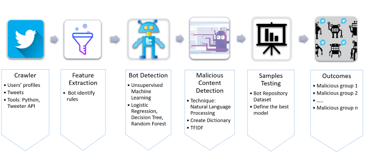
Coming into this project, we did some research and decided to divide the process into two phases. Before the implementation, we used Python to scrape account metadata and tweets of Twitter bot IDs. During phase one, we applied supervised machine learning to train Decision Tree, Random Forest, and Logistic Regression with behavioral bot features. In phase two, we engineered new features from tweets using Natural Language Processing and trained the models again. The result was amazing! We built a Random Forest classifier with 91.68% of accuracy (for testing data).
APPROACH
Here is our pipeline:
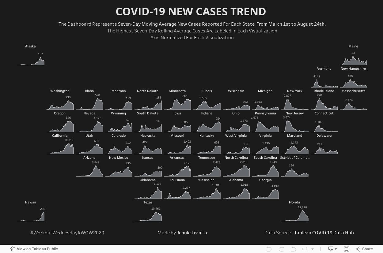
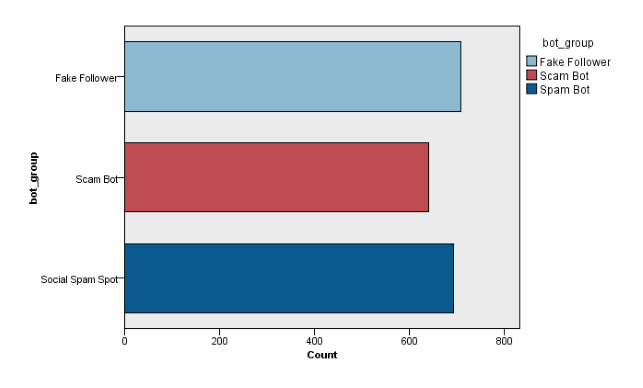
The raw dataset included 900 IDs for each kind of malicious bots from Bot Repository, total 2700 IDs. After scraping account metadata and tweets with Twitter API and Tweepy, we visualized number of tweets collected in the following graphic.
PHASE ONE: SPOT A BAD BOT BY BEHAVIOR
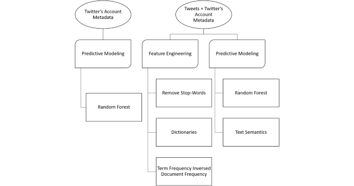
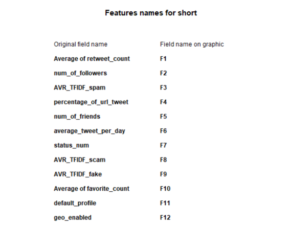
We used IBM SPSS to build an uncorrelated forest of trees to predict the type of malicious bots based on 13 identified fields of account's behaviors. The features included average retweet per ID, average favorite per ID, bot types, bot groups, number of followers, number of friends, number of tweets per ID, a binary feature of default profile (yes/no), a binary feature of using default profile image, if geo-location is turned on, average number of tweets posted daily per account, and percentage of tweets containing URL or hyperlink for each account.
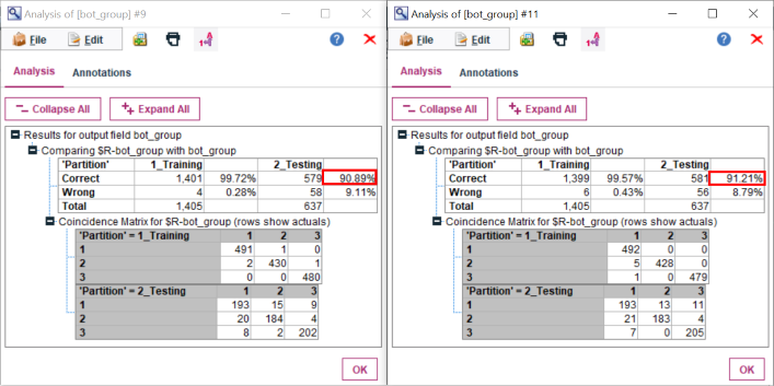
We partitioned data into 70% of the training set and 30% of the testing set. The Random Forest predicted bots 99.43% correctly on training data, and 91.05% correctly on testing data. The Random Forests Classification indicated that some features matter more than others. Retweet frequency, number of followers and daily tweet frequency were identified as top 3 important features.
PHASE TWO: SPOT A BAD BOT BY BEHAVIOR AND TWEET SEMANTICS
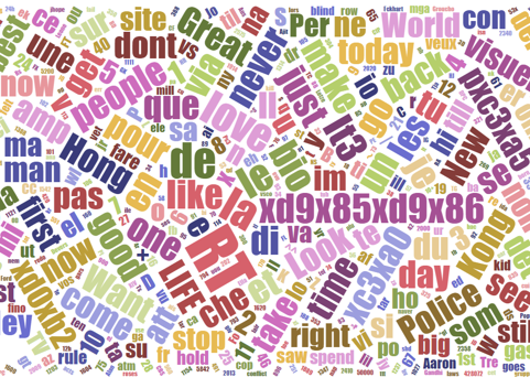
We used Natural Language Toolkits to get keyword dictionary and keyword frequency for 216,173 tweets. We calculated every term frequency for each group of malicious bots. With the 0.05% threshold for term frequency rate, terms larger than the threshold were selected to create detection dictionaries for fake followers, scam bots, and spam bots. We used Python and Excel to calculate they keywords' TFIDF in each tweet using three dictionaries. Then we normalized TFIDF of each tweet to make sure they had the same weight and calculated the average normalized TFIDF for each account. We visualized the term frequency with WordClouds to make sure that the results were consistent with the TFIDF calculation.
In short, fake followers have the lowest TFIDF score in all three dictionaries and a little better match in fake follower dictionary due to their small number of tweets. Scam bots have high TFIDF in all three dictionaries and especially in the spam dictionary. Spam bots do post tons of tweets, and the result indicates that there are some words in the spam dictionary that have discriminative power to distinct spam bots from other types. We added these three average TFIDF as our new features in our detection model and built a new model to see whether these three new features can contribute to our overall accuracy.
Spam bot's Tweets WordCloud
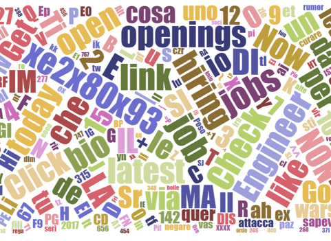
Scam bot's Tweets WordCloud
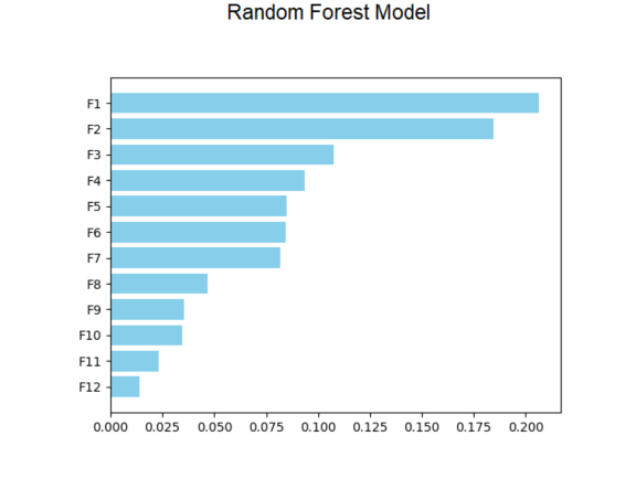
The Random Forest Classification applied 12 inputs as predicting factors to train 1405 records again. The dataset was partitioned into 70% of the training set and 30% of the testing set. Adding three new inputs of average TFIDF scores of fake followers, scam bots, and spam bots, the model produced a new list of important indicators. The top three indicators were the average of retweet frequency, the number of followers, and average TFIDF score of the spam bot. According to the result, the TFIDF score plays a significant role in classifying types of malicious bots. This new model predicted malicious bots correctly of 91.68% on the testing set.
MODEL EVALUATION
The model in phase two performed slightly better than the model in phase one. Obviously, the TF-IDF features certainly contributed to the improvement of the model.
WRAPPING UP
You made it here !!! To snapshot the process, we combined supervised machine learning and natural languague processing to detect malicious bots on Twitter.
Overall, fake followers are inactive accounts with the highest TFIDF score for fake accounts. Scam bots are also inactive accounts but they retweet frequently and have the highest TFIDF score. Spam bots are active accounts with the highest TFIDF score.
Thanks for reading!
SPOT A BOT THROUGH VISUALIZATION
If you want to understand how different bots behave on Twitter, check this Viz out!
Recommendation Systems are very standard and popular all over the web. Companies like Netflix, Spotify, Apple, Pandora, and LinkedIn leverage the recommender systems to help users find new items quickly, creating a delightsome user experience while driving incremental revenue.
Available on Github.
BIG PICTURE
Discover Playlist is one of the most popular Spotify’s features, and it is generated each week based on user’s listening habits. Inspired by this playlist, I and three other classmates geeked out about recommendation algorithms and decided to create three music recommendation systems for our Big Data capstone project.
We employed three algorithms (popularity benchmark, ALS, lyric-based and artist-based similarity filtering) to generated three different playlists: Hot Song playlist, Personalized playlist, and New User playlist. ALS algorithm was used for a personalized recommendation. The lyric-based and artist-based similarity algorithm was used to solve the cold-start problem with new users.
The whole system was built with Python and PySpark on Google Cloud Platform and AWS.
ABOUT THE DATA
The Million Song Dataset, a collaborative project between The Echo Nest and LabROSA, is a freely available collection of audio features and meta data for a million contemporary popular music tracks.
The links are available here:
Taste Profile, The musiXmatch dataset, The Million Song subset
APPROACH
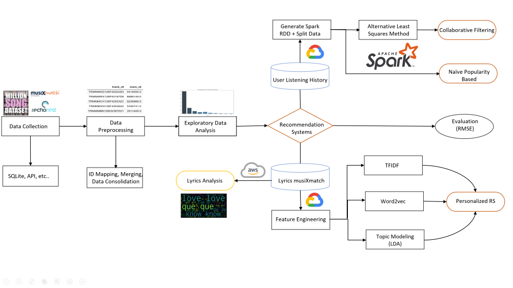
ALGORITHM DEVELOPMENT
1. Popularity Benchmark
Popularity is the benchmark for recommending songs because it is better than random guesses. The data were filtered by total frequency based on listening history, then top 10 heated tracks were selected. This would be the baseline saver in case there is no data for a new user (cold-start problem).
2. Collaborative Filtering
Collaborative filtering is probably one of the most used approaches for the recommendation system, or at least as a necessary component of some advanced recommendation structures. Surprisingly, this algorithm requires such simple data, nothing more than the users’ historical preference on a set of items. The main assumption here is that the users (listeners in our case) who have agreed in the past are very likely to agree in the future. For multiple users, it assumes if user A liked the same product as user B, A would also like to have similar taste as B for other B’s favorites.
In terms of the ratings, the algorithm often requires some metrics to indicate users’ preference, which can either be explicitly available data such as 5 stars or thumbs-up on the product, or an implicitly derived score such as clicks, number of purchases, or other data recorded in the cookie. In this project, traditional way was implemented by utilizing the listening frequency as the rating. The assumption when lacking explicit rating is that a higher listening frequency equates to a higher rating.
For ALS, a matrix with frequency of each song played by each user was constructed. Certainly, this matrix is sparse with tons of missing value, as a limited number of users have listened to only a limited set of songs. The high-level idea is to approximate the matrix by factorizing it as the product of two matrices: the user matrix that represents each user, while the item matrix describes properties of each track.
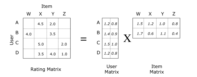
For a reasonable result, two matrices were created so that the error for the known user-song pairs is minimized. The error here refers to the rooted mean squared error (RMSE). In a more detailed technical level, ALS would first fill the user matrix with a random value, and then optimize the song matrix value by minimizing the error. After that, it “alters”, which means it would hold the song matrix and optimize the value of the user’s matrix. This step minimizes two loss functions alternatively and should achieve some optima.
During the implementation, Spark ML pipeline was used with the following settings:
- A big set of the parameters were picked and grid-search with cross-validation on this space was executed.
- Some important parameters to tune include: maxIter (the max number of iterations), rank (the number of latent factors, which basically determined the shape of matrix), and regParam (the regularization parameter).
3. Content-Based Filtering
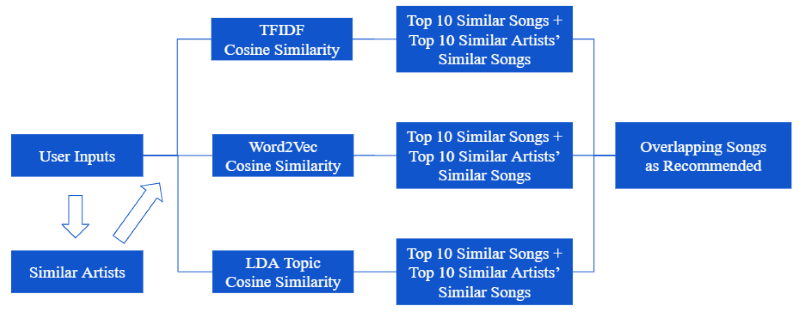
Content-based filtering generates song playlists based on the cosine similarity calculated for three lyrical features, including (1) TF-IDF, (2) Word2Vec, and (3) Topic Model with Latent Dirichlet Allocation (LDA).
In this case, the algorithm is designed for new users to search for a specific song. The users enter their favorite song or artist, then the system will match the song’s index with cosine similarity matrix and return 10 songs with similar content.
TFIDF for Lyrics: TF-IDF stands for “Term Frequency – Inverse Document Frequency”. In this case, we vectorized the lyrics and use TF-IDF to quantify the word in song lyrics. We computed a weight to each word which signified the importance of the word in the lyrics.Because the actual lyrics were protected by copyright and Million Song Dataset did not have permission to redistribute them, the lyrics came in the form as bag-of-words rather than the original lyrics. This created limitation to this approach.
Word2Vec for Lyrics: Word2Vec is a two-layer neural net that processes text by “vectorizing” words and turns text into a numerical form. Word2vec groups vector of similar words in vector space as it detects similarities mathematically. Due to high volume of data, calculating the cosine similarity using high-dimensional sparse TFIDF matrix was time-consuming and costly. In this case, Word2vec was used as the second method. However, Word2Vec model was less accurate because there was no context due to lyric limitation.
LDA for Lyrics: Topic Modeling is an unsupervised approach used for identifying topics present in a text object and to derive hidden patterns exhibited by a text corpus. Latent Dirichlet Allocation (LDA) is one of the topic models that builds a topic per document model and words per topic model. The big idea behind LDA is that each document can be described by a distribution of topics, and each topic can be described by a distribution of words.We assumed that there are similar topics among all songs and limited the number of topics to help save time and memory. LDA was used as the third method. In this case, LDA ignored syntactic information and treated documents as bags of words, so the unigram format in the dataset did not matter much.
Artist Similarity: The dataset is offered by Million Song Dataset. We assumed that similar audience would have the same taste in artists.
After engineering new features and calculating the cosine similarity between them, we defined two key functions for our recommendation system. One returned the top 10 song with the highest cosine similarity. The other found the top 10 songs based on artist similarity and cosine similarity.
RESULT AND EVALUATION
1. Collaborative Filtering
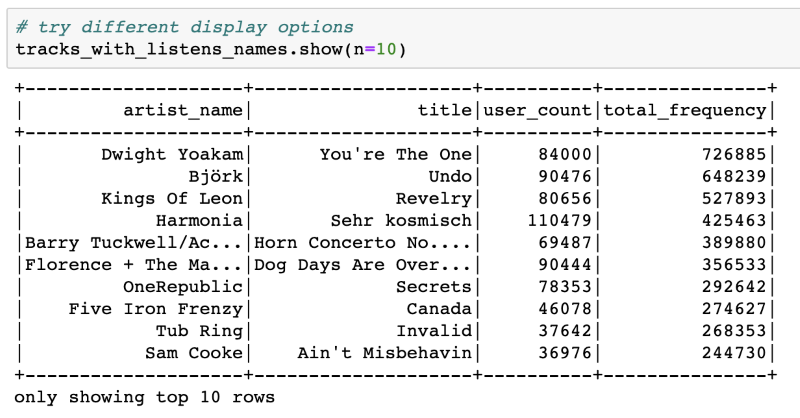
Here is the benchmark of our top 10 most listened songs.
The data was split into three parts: 60% as train, 20% as validation, and 20% as test. Grid search and cross-validation on validation set was implemented to determine the best parameters of the recommendation system and only recommend the results to the new users in the test set once to avoid information leakage. The process was implemented from scratch and was locked in a pipeline. This work was constructed to avoid overfitting problems.
As for Spark 2.0, when asked to provide a rating for new users never seen before, the ALS could only yield NAN value. . Therefore, it was impossible to adapt Spark ML’s Cross Validator to check the RMSE. So the algorithm was set to drop NAN values by default with customized cross validation process before using RMSE for evaluation.
The following configuration steps were executed: (1) set appropriate parameters for users, items and rating; (2) fit ALS and transform the table to generate the prediction column; (3) run predictions against the validation set and check the error; (4) finalize the model with the best RMSE score.
Exploratory analysis showed that more than half of the songs in the sample were listened at least once. Thus, it could be inferred that songs played more than once can better represent users' tastes and run the ALS on two versions of the datasets.
Result comparison of model with all data and frequency >=2 data was shown as followed:
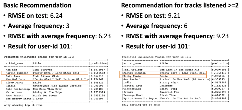
Except for cross-validation, another common measurement is to compare the model with fake test data where every rating is the average number of frequencies from the train data. While the model excluding the 1-time listened songs returns a slightly higher RMSE score on the test dataset, it behaves better when compared with the average frequency. And this may hint the recommendation makes more sense. The highlighted tracks can be of the highest recommendation quality, as they are the overlap between two ALS recommendation models.
2. Content-Based Filtering
Let's simulate a new user searches for a song to see the recommendation results.
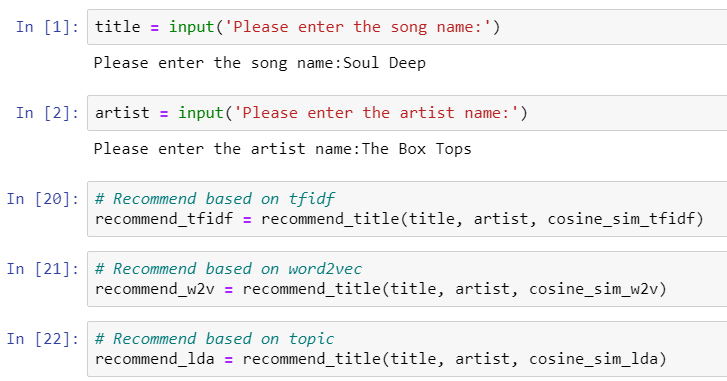
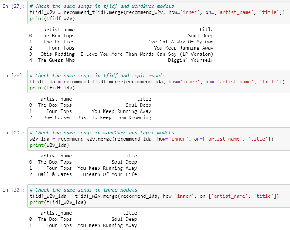
The results showed: 4 similar songs between TFIDF and Word2vec methods; 2 similar songs between TFIDF and LDA methods; 2 similar songs between Word2vec and LDA methods; 1 similar song among three methods. Therefore, the final recommended song related to the Box Tops’ Soul Deep was Four Tops’ You Keep Running Away.
BEYOND THE LYRICS: THE CROSSROAD OF MUSIC AND DATA VISUALIZATION
Always amazed by the power of data visualization, I wanted to bring the hidden trends in the meaning of songs to light. Additional to building music recommendation systems, I utilized Natural Language Processing, WordClouds and seaborn to investigate the popularity of lyrics from 1950s to 2000s as well as the topic in lyrics.
1. Topic Modeling Visualization
When modeling lyrical topics with LDA, lyrics were not stemmed, and the model defined 20 topics. The original word form was kept for more comprehensive analyses. I removed stop-words, generated token dictionary, and built a corpus. Then the corpus and dictionary were filtered into the LDA model with 20 topics.
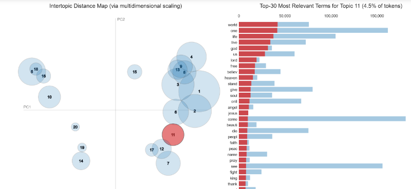
Cluster 5,10,18, and 16 as well as cluster 20,19 and 14 were separated from other clusters in different dimensions due to the difference of languages.
Cluster 11, 17, 12, and 7 contained lyrics of violent or religious topics. For instance, cluster 11 represented religious topic with the most relevant words of “world”, “life”, “live”, “god”, “us”, “heaven”, “god”, “Jesus”, “soul”, “angle”, and many more. However, topic in cluster 12 seemed to be related to violent topic, or rap song, since the lyrics contained very negative words, such as the “f” word, “kill”, “dead”, “hate”, “hell”, “gun”, “shit”, “bitch”, “war”, “sick”, “shot”, or “murder”.
The first dimension (upper right side) included topics with positive vibe, such as love or party. For instance, cluster 15 seemed to have a “dance party” theme with mostly “oh”, “ooh”, “ah”, “yeah”, “shake”, “mama”, “yes”, “babi”, “ohh” and so on.
Multiple clusters with “love” topics were blended because “love” intuitively brings out many emotions. For example, cluster 8 seemed to represent “happy love” with “love”, “want”, “need”, “feel”, “like”, “kiss”, “true”, “touch”, “give” and so on while other clusters represented sadness.
In general, a good class of 20 topics could be defined with the LDA model. Each topic was approximately well-defined with different themes, such as religion, dance party, dark drama, happy love, and sad love.
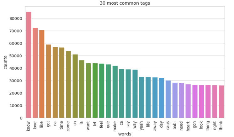
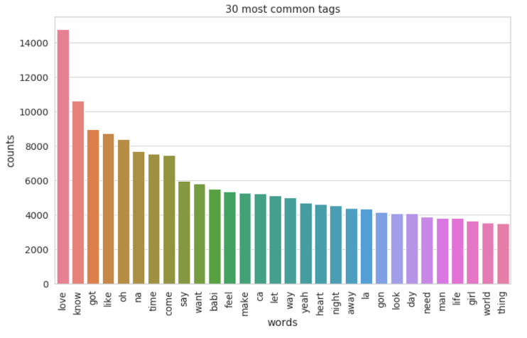
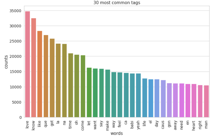
2. Lyrics Analysis Through The Time
There are certain changes in lyrics from 1950s to 2000s:
"Love" was the most used word in songs from the 1950s to 1990s. The topic of love seemed to be the greatest inspiration for music at the time. In 2000s, "know" became the most used word and followed by "love".
The party vibe was shown more frequently in 1990s and 2000s. Those words such as "got", "na", "like", "oh", "la", "come", "let", "feel","make", and "yeah" became very popular in lyrics.
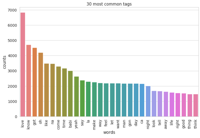
Though songs of 1950s and 1960s sounded more conservative yet filled with romantic vibe. The popular words were "girl", "time", "night", "make", "say", "day", "want","heart", "man", and "said".
The word "babi" was in the top 3 popular words in 1950s, however, from 1960s to 2000s, it was replaced with either "like" or "got".
Lyrics in 2000s:
Lyrics in 1990s:
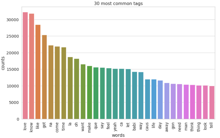
Lyrics in 1980s:
Lyrics in 1970s:
Lyrics in 1960s:
Lyrics in 1950s:
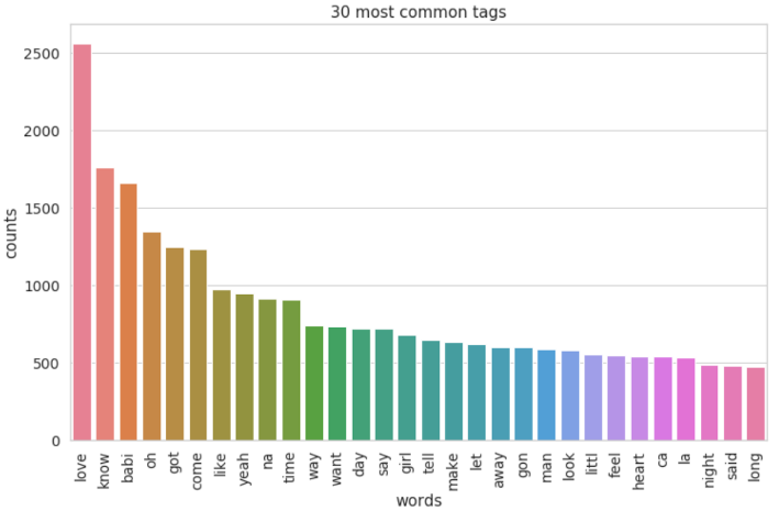
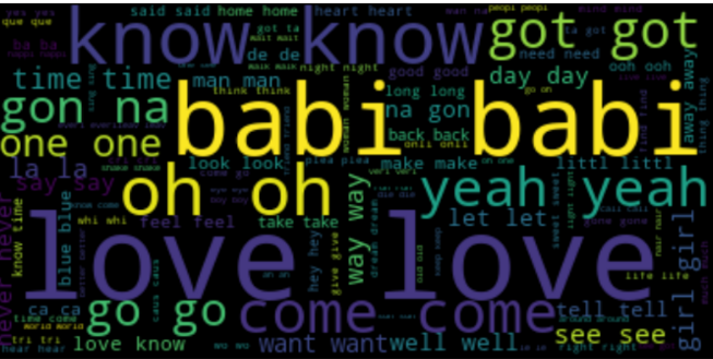
Comparing the most popular words in lyrics of the 60s and 2000s, the lyrics in the 60s tended to bring a more subtle vibe than the 2000s did. The 60s lyrics had “babi”, “know”, “love”, “yeah”, “oh”, and “got”, which demonstrated the priority in love and the lover. At the same time, the 2000s lyrics had “love”, “la”, “know”, “got”, “de”, and “come”, which portrayed a bustling vibe and prioritized love and party at the same time.
Word Cloud for Lyrics in 1960s:
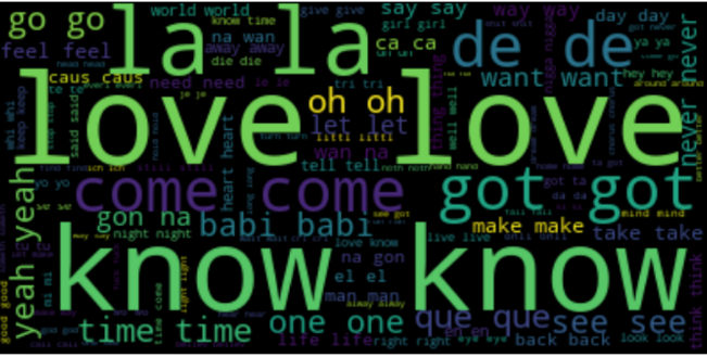
Word Cloud for Lyrics in 2000s:
CONCLUSION
In this project, three recommendation systems were built using a dataset with 1,019,318 unique users and 384,546 unique songs. ALS algorithm, which combines user and item knowledge, was used for collaborative filtering recommender. This recommender can be applied to old users with sufficient listening history to generate personalized recommendations. Many features of song were combined, such as artist similarity, TF-IDF, Word2vec and LDA modeling for lyrics, to build a content-based recommender. The content-based recommender is for new users with only one or a few searches and listening history. Similar songs for the current song will be recommended. Considering that Spotify has about 2 million monthly active users, our project is close to the monthly magnitude of the industry-level. Yet a lot of obstacles during the implementation process still emerged.
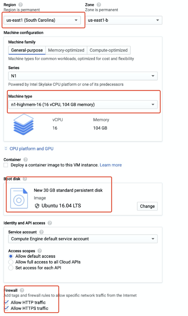
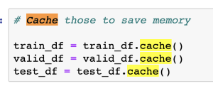
There are many lessons can be learned when working with Cloud and Pyspark. First, Spark has a high dependency on memory usage. During the testing phase, our virtual instance with 30GB memory crushes from time to time. It would save some cost to choose a high memory specialized instance on google cloud. To run cross validation on the 3GB listening history data, it would be secure to choose the following configuration. It is very helpful to use the Unix command “free -m” to check available memory in time. In addition, we learned that we need to cache the datasets whenever they are likely to be used more than once:
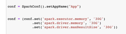
However, overcoming memory issues on cloud alone is not sufficient. Some default Spark settings needed changing to permit more executing memory and driver memory resources to be adapted by Spark.
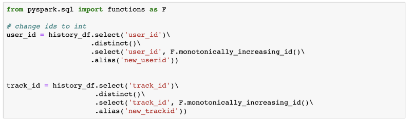
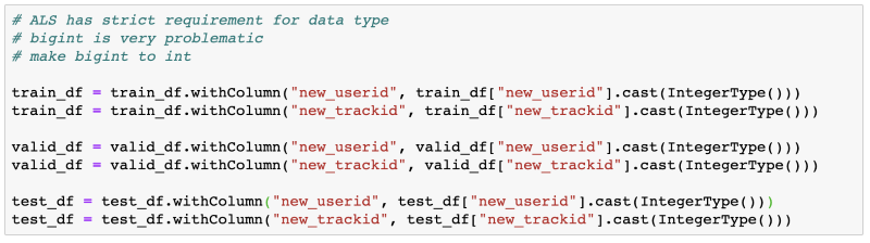
In addition, debugging with Spark is quite suffering, as the error message is not informative enough. A common mistake is that the data type is not fixed or switched during the processing. Due to the Java development environment, different methods are very strict on input data type. Casting the data types should be a regular task while working with Spark. For example, ALS function in spark only allows integer input. It would return error even when the data type is big integer and so on. In the same vein, the raw ideas from the original data frame are no longer useful that new integer id pairs have to be generated.
An example of change the Data Type to Int:
An example of change ID's Data Type from Bigint to Int:
Curently, there are still obstacles towards a final hybrid recommendation system. At this stage, the main difficulty comes from the lack of valid lyrics data. In the future, combining the collaborative filtering and content-based recommendation systems can provide hybrid recommenders. According complementary advantages from various recommendation algorithms, hybrid solution, such as using overlappings, would provide users with suggestions of higher quality.For example, a hybrid system based on lyrics and listening history could make sure the users like not only the explicit topics of the tracks but also the genre from their taste perspectives.
As a matter of fact, more dimensions of recommendation are always better. Google naturally combined plenty of recommendation strategies in its wide and deep recommendation system with neural networks and ensemble methods. Though it is difficult to bring this project to such a top level, this precious practice undoubtedly helped lay a solid foundation for potential industrial workds involving recommendation systems or distributed systems.
Besides, there are some new ideas for further exploration:
1. User2Vec:
Word2Vec for NLP was used in this project to analyze the knowledge about songs. What if songs are considered as words and users are considered as documents? The listening history of a user is the text content of the document. Then Word2Vec and Doc2vec can be applied to find similar songs and users.
2. Graph algorithm:
Graph database is another new trend for online shopping recommendation systems. When modeling songs, artists, and users in a graph database, graph algorithms can help to find the relationship among those features and consider knowledge about songs, artists, and users at the same time.
3. Content-based filtering using music audio:
In this project and the lastest business scenarios, content-based filtering in the music industry means lyric-based or text-based. However, machine learning and and deep learning also show great results and improvements in audio processing. Analyzing the music audio directly could be a new direction for content-based filtering.
REFERENCE
1. A Beginner's Guide to Word2Vec and Neural Word Embeddings. (n.d.). Retrieved from https://pathmind.com/wiki/word2vec
2. Content-based Filtering. (2012, January 24). Retrieved from http://recommender-systems.org/content-based-filtering/
3. Karantyagi. (n.d.). karantyagi/Restaurant-Recommendations-with-Yelp. Retrieved from https://github.com/karantyagi/Restaurant-Recommendations-with-Yelp
4. Li, S. (2018, June 1). Topic Modeling and Latent Dirichlet Allocation (LDA) in Python. Retrieved from https://towardsdatascience.com/topic-modeling-and-latent-dirichlet-allocation-in-python-9bf156893c24
5. 5. MODELING. (n.d.). Retrieved from https://xindizhao19931.wixsite.com/spotify2/modeling
6. Welcome! (n.d.). Retrieved from http://millionsongdataset.com/
Every March, millions of basketball fans, celebrities, data scientists and even presidents tune in to watch and predict the championship of NCAA Division I Men’s Basketball Tournament. Excited by all the odds of filling out a perfect bracket, I joined the annual March Data Crunch Madness competition, hosted by Fordham University and Deloitte. Even though the NCAA cancelled the tournament because of COVID-19 in 2020, I, and other participants still decided to try our hand at modeling the tournament and kept the tradition at Fordham going.
Available on Github.
BIG PICTURE
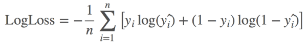
The goal of the competition is to utilize past tournament data (from 2002 to 2019) to build and test predictive models in order to forecast outcomes of the Final Four in the 2020 NCAA Division I Men’s Basketball Championship. These outcomes are computed probabilistically, and the models are evaluated by log loss. For instance, Team 1 has 70% likelihood of winning Team 2. Also, if you are not familiar with log loss, just know that the best model has the lowest log loss.
APPROACH
Coming into this competition, I did some research on similar projects and came up with a general idea of what to do. As far as I knew, some projects went with logistic regression as their primary algorithm because of the probabilistic nature and simple implementation, yet effective. With my prior knowledge, I took a similar approach to other models while making a few interesting changes with novel features.
So, what is new about my approach?
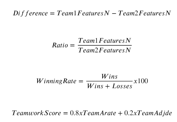
Instead of analyzing the stats of each team, I engineered new features by transforming all variables into Difference and Ratio, or Quotient, between two teams in each of 63 games.
Then I calculated the Winning Rate and Teamwork Score for each team and coach. The level of teamwork can be reflected by the percentage of assist score (80%) and the defensive efficiency (20%). The team can be more stable if they rely on assist and better defense to win the game.
To select the most important features, I removed highly correlated variables (Pearson correlation > 0.9) and applied Embedded method with Random Forests. Some advantages of Embedded methods are higher accuracy, better generalization, and being interpretable (based on importance). Also, it works well when dealing with high-dimensional dataset.
After hyperparameter tunning Random Forest Classifier with Grid Search, I trained Logistic Regression, Gradient Boosting, Support Vector Classifier, Random Forest Classifier, and Linear Discriminant Analysis (LDA) and selected the best one with lowest log loss.
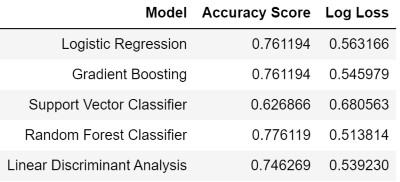
MODEL SELECTION
Random Forest Classifier is selected as the best model due to the most optimal accuracy rate and lowest log loss. That should be enough for the competition. The perfect scenario was having the 2020 data for model application. However, to resolve the problem, I trained the models with 2002 to 2017 data, tested the models with 2018 data and then I applied the model on the 2019 data to generate prediction and probability.
PREDICTION RESULT
The accuracy of the best model Random Forest Classifier is 77.61% with a log loss of 0.51.
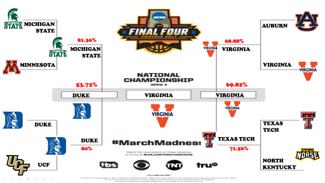
So which teams are the final four and champion?
WRAPPING UP
I am happy to say that completing this competition has made me a more competent data scientist, especially under the unprecedented situation. I am excited and hopeful that the 2021’s tournament will not be cancelled so I can make some fun bets with my friends using this model. Thanks for reading and if you want to learn more about my code, please visit my github.
MARCH MADNESS VISUALIZATION
If you are interested, here are some interesting visualizations about March Madness! See if you want to make a bet for Virginia !
